Old News
Quick Tutorial on Using Information Miner
All the underlying algorithms are implemented as native console applications. You can find a tutorial for using these tools directly here. Since all tools use an interchangeable text format to store their results it is possible (and intended) to chain tools together. Information Miner serves as a graphical frontend to aid in this respect.
Let's solve exercise 25.
Starting Information Miner
Download the binary package. It is a self-contained jar file and contains everything, so you don't need to worry about missing libraries or class paths. Java version 1.5 is required. For the time being this version contains only the Windows executables of the tools. If your are using another operating system, you will have to use the tools at the command line as described under the above-mentioned link.
Start Information Miner by double clicking the jar file or type
java -jar InfoMiner-2.0.jar
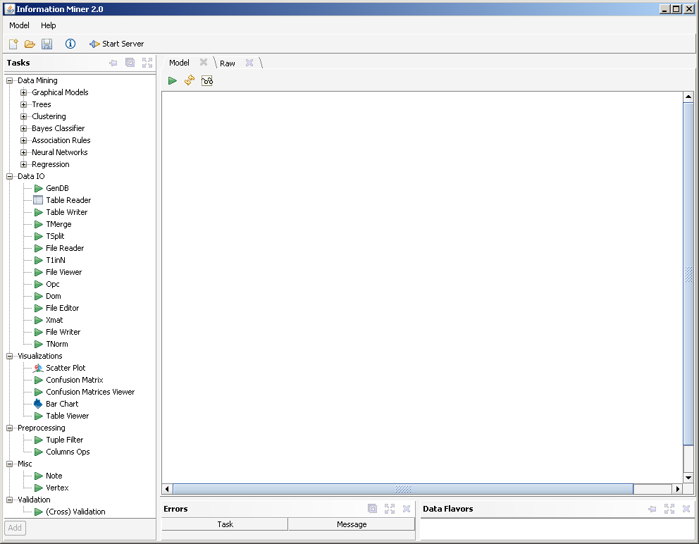
at the command line. You should see the following screen:
Getting and Setting the Input Data
Download the input data (the table given on the exercise sheet). It is a simple space-separated file with a header.
In Information Miner, drag and drop a "File Reader" from the left panel to the right empty area. (don't be confused that it reads "iris.tab", that is a default value) You can zoom in and out using the mouse wheel. Panning the entire content is done with the right mouse button pressed.
Now right click on the file reader and choose "Customize..." (or just double click on it). Click the "..." button and choose the just downloaded "train-25.tab". You may use "Preview" to confirm that you chose the correct file; it will only show the first ten lines though.
Setting Up the Classifier
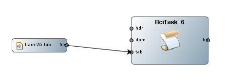
Drag and drop the "Bci" icon from the left pane onto the working area. You may need to expand the "Bayes Classifier" node. "Bci" stand for Bayesian Classifier Induction which is exactly what we want. As you can see, the Bci task has three input, two of which are mandatory: tab and dom. The tab input is simply our data file. Click on the output "file" of the file reader, and drag it to the input "tab" of the Bci task until it snaps in. The result should look like this:
However, up to now, the Bci task does not know what kind of data type it has to expect. Remember that such a classifier can deal with nominal data as well as with metric values. To advice the type of the domains of the attributes (here: x, y and Class), we need a "domain file" or dom file for short. We could write it by hand but we use automatic induction here.
Drag a "Dom" task to the working area. Connect the file reader output to the dom task's tab input. To look at the domain file, create a "File Viewer" and feed into it the dom output.
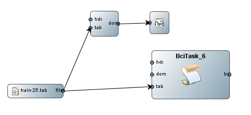
Run the file viewer by right clicking on it and choosing "Run". It will start a task cascade and pop up a text window with the following content:
    /*----------------------------------------------------------------------
      domains
    ----------------------------------------------------------------------*/
    dom(x) = { 3, 4, 5, 6, 7, 8, 9, 1, 2 };
    dom(y) = { 1, 2, 3, 4, 6, 5, 7, 8, 9 };
    dom(Class) = { a, b };
Obviously this is not what we want since the dom task treated all attributes to be nominal and thus exhaustively lists all values. To advice it to automatically try to detect the type close the text window an double click on the dom task. Enter "-a" into the "params" field and click OK. Now reset the dom task by right clicking on it and choosing "Reset". Again, run the file viewer task. It should now present a correct domain file:
    /*----------------------------------------------------------------------
      domains
    ----------------------------------------------------------------------*/
    dom(x) = ZZ [1, 9];
    dom(y) = ZZ [1, 9];
    dom(Class) = { a, b };
Now, the domain file correctly tells that x and y are integers in the range of 1 and 9. The Class type has not changed since it is nominal.
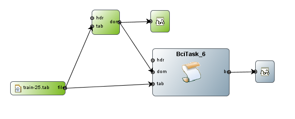
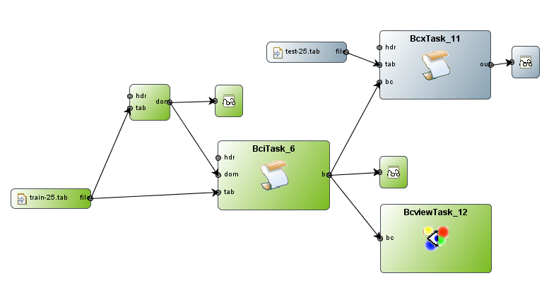
Feed the domain file into the dom input of the Bci task and also connect a new file viewer to the bc output.
Run the Task
We are now ready to execute the induction of the classifier, so right click on it and choose "Run". To look at the textual representation run the attached file viewer.
    /*----------------------------------------------------------------------
      domains
    ----------------------------------------------------------------------*/
    dom(x) = ZZ [1, 9];
    dom(y) = ZZ [1, 9];
    dom(Class) = { a, b };

    /*----------------------------------------------------------------------
      naive Bayes classifier
    ----------------------------------------------------------------------*/
    nbc(Class) = {
      prob(Class) = {
        a: 10,
        b: 10 };
      prob(x|Class) = {
        a: N(5.6, 4.48889) [10],
        b: N(4.2, 4.62222) [10] };
      prob(y|Class) = {
        a: N(3.7, 3.56667) [10],
        b: N(6.4, 3.82222) [10] };
    };

    /*----------------------------------------------------------------------
      number of attributes: 3
      number of tuples    : 20
    ----------------------------------------------------------------------*/
You easily verify the parameters we calculated manually in the exercise lesson. The parameters include the class distribution (uniform here) and four class-dependent Gaussian distributions.
View the Classifier
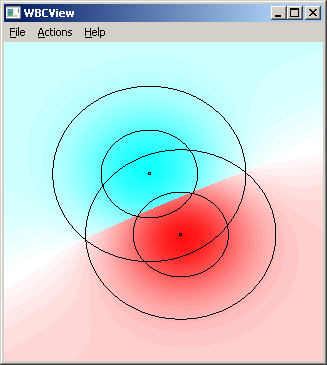
To get a visual representation, create a "Bc Viewer" task and feed in the bc output. Run it and you will get the normal densities of the respective classes:
Use the Classifier
To finally use the classifier for classification, download the test data file and create a new file reader for it.
Create a "Bcx" task (Bayesian Classifier Execution) and set it up with the classifier just learned. Double click on the bcx task and enter "-ax" to the params field. This tells the task to align the output fields and print additional probabilities to the output. Feed the output of bcx into a new file viewer. And, of course, do niot forget to connect the test file to the bcx task:
Now run the last file viewer to start the task cascade. The output shoud read:
    x y bc a     b
    8 7 b  0.375 0.625
    3 4 a  0.548 0.452
The columns x and y are just repeated. Column "bc" represents the predicted class. The last two columns show the calculated probabilities that led to the prediction. These are the same probabilities as calculated during the exercise lesson.
Hint for exercise 26
Exercise 26 asks you to learn a full bayesian classifier. You can check your manual calculations by advising the bci task to learn a full one. This is done by entering "-F" into its params field.

